How to reach the top of the imagenette leaderboard?

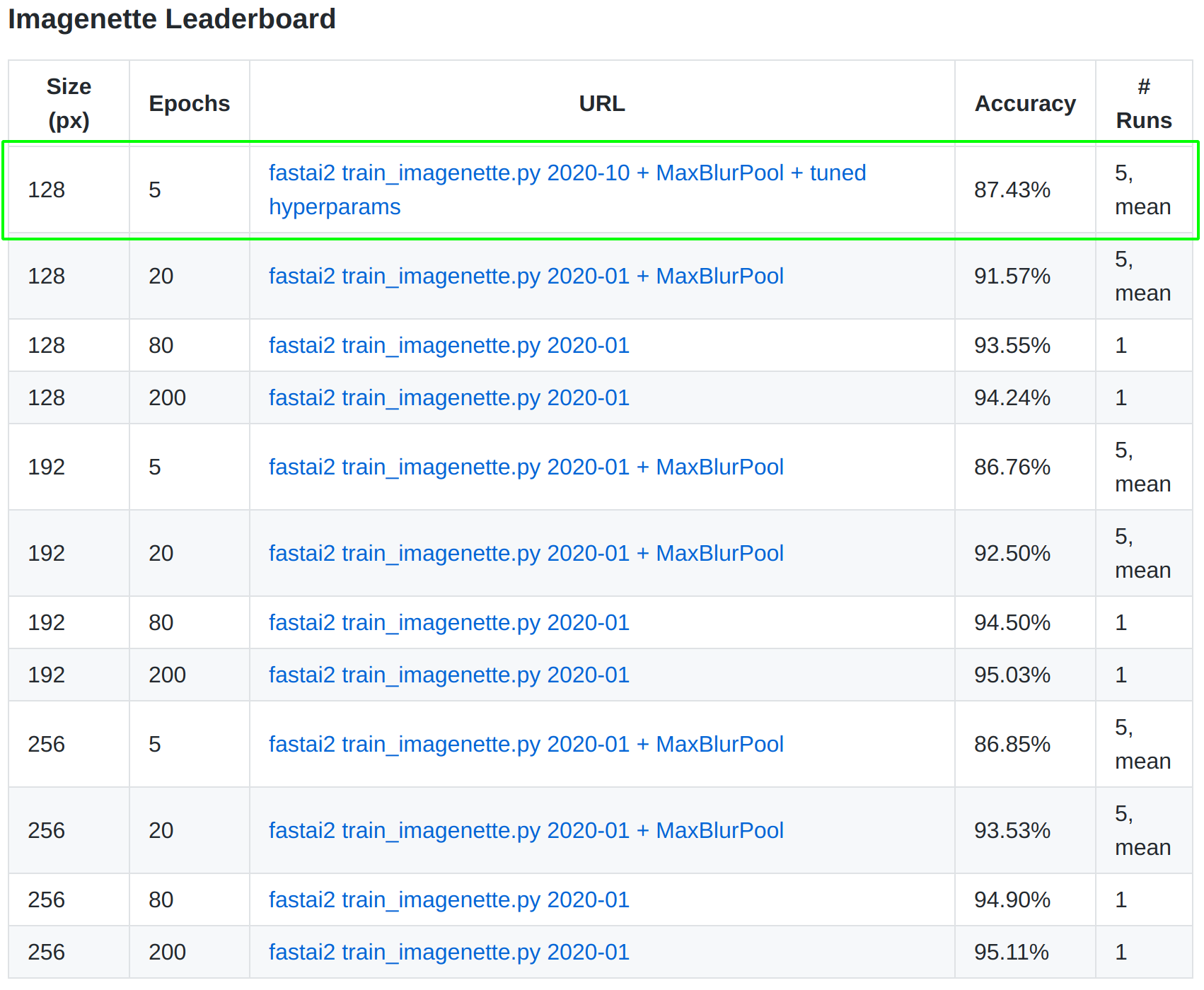
In my solution, I combine insights from submissions by Dmytro Mishkin and Peter Butterfill and perform hyperparameter optimization to reach first place on the leaderboard.

In this article, we will take a closer look at:

• BlurPool — a way of combating aliasing that makes neural networks more robust to small image shifts (it provides a significant performance gain)
• hyperparameter tuning and the reasons for the suggested parameter changes

The task for which I reached the top of the leaderboard is the top 1 accuracy on imagenette with an image size of 128px and number of epochs equal to 5. Please find the code I used for my submission here.

What is imagenette?

It is a subset of 10 easily classified classes from Imagenet (tench, English springer, cassette player, chain saw, church, French horn, garbage truck, gas pump, golf ball, parachute) that is made available by fast.ai.

Given its nature, this dataset lends itself very well to quick experiments and the study of new methods. The leaderboard provides a nice way of evaluating how your approach is doing, whether you are on the right track, plus it contains links to working implementations!

Imagenette can be found on GitHub here.

BlurPool

A factor contributing very strongly to the performance of the model that I trained  is BlurPool introduced by Richard Zhang in the Making Convolutional Networks Shift-Invariant Again paper.

This is a brilliant technique that addresses a rather surprising shortcoming of modern CNN networks. Turns out they are not shift-invariant after all and are so by design (earlier methods of addressing this issue reduced performance and were discontinued).

Shifting the input image by just one pixel can lead to startlingly different predictions!

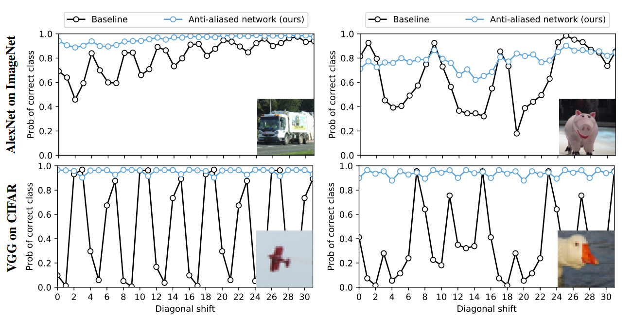
The above figure from the paper, in the bottom left-hand corner, depicts what will happen to the predicted probability of the correct class for a tiny image of an airplane as we continue to shift the image sideways. A shift by just a single pixel can bring the predicted probability of the correct class down from nearly 1.0 to around 0.2.

VGG is particularly affected by this phenomenon, but other CNNs suffer from this as well.

Here is a brief outline of what is going on.

As we apply transformations to the image and subsequently the feature maps, we ignore the sampling theorem! In the process, we incur aliasing - the same signal can create varying representations if shifted!

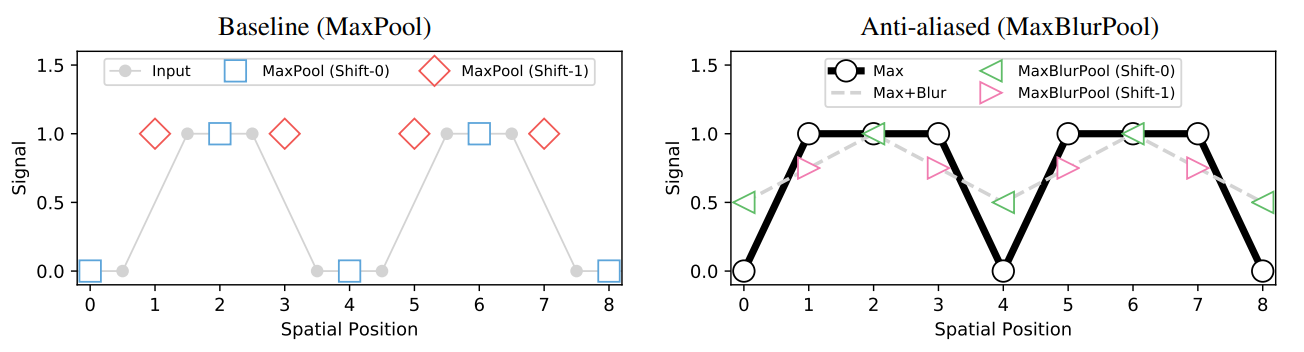
The above figure from the paper demonstrates this effect very well

In modern CNNs, MaxPool is the main culprit contributing to this effect.

The proposed method doesn't entirely remove the issue, but — as depicted in the figure above on the right, it makes the problem much less pronounced.

To be honest, I have not come across the application of the Nyquist frequency to images before and I find this topic fascinating. The discussion in the paper is both very elegant and very interesting to read.

If you would like to learn more about how convolutions can be used for blurring (or the application of some other effect), I would recommend this wonderful video.

Let us now take a look at some of the hyperparameter changes I introduced and the reasoning around them.

Hyperparameter optimization

With that low number of epochs (only 5, that is very little given that we are starting with randomly initialized weights), this task is in its essence a race to a good set of weights.

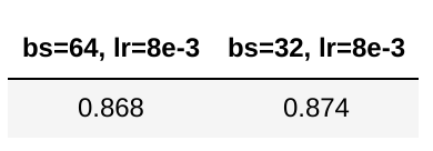
As such, it is a good idea to change the batch size from 64 (which some of the earlier models were trained with) to 32 while keeping the learning rate constant.

The lower batch size will allow for twice as many weight updates during training, though each of the updates will not point as precisely towards a minimum as it would be the case with larger batches.

Nonetheless, for this particular situation (and as is often the case when we are limited in how long our training can take), taking a higher number of steps in the weight space improves results.

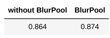
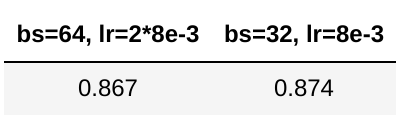
One might make an objection that the value of the learning rate is only meaningful in the context of the batch size. Here, one could argue that when training with a lower batch size, we are effectively training with a higher learning rate. This would be correct, but as evidenced below, even if we linearly scale the learning rate to adjust for the differences in the batch size, we still get a decreased performance with a smaller number of steps.

Further to that, as we are rushing towards a solution and the total number of epochs is relatively low, we do not need to worry too much about overfitting. As it turns out removing data augmentations (RandomResizedCrop  → Resize, disabling RandomErasing) leads to a better result.

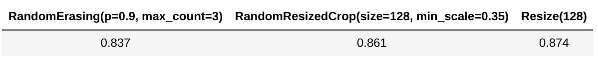
This result intuitively makes sense. Data augmentation does come at a cost. It makes it harder and slower to train our model, but it also allows us to make better use of our model's capacity with more training (as evidenced by other results on the leaderboard and cursory tests I ran that I do not report here).

Other techniques

My intention behind writing this blog post was to highlight the techniques above. Nonetheless, for the sake of completeness, I include a brief mention of some of the other techniques and architecture modifications that went into the training of these models and that are available from the fastai library out of the box. Please note that the list is not exhaustive.

• ResNext — architecture modification applying the split-transform-merge strategy from Inception models to resnet architectures in a modular fashion
• Improved CNN stem and path-dependent initialization (Bag of Tricks for Image Classification with Convolutional Neural Networks)
• The Ranger optimizer — a synergistic optimizer combining RAdam (Rectified Adam) and LookAhead, and now GC (gradient centralization) in one optimizer
• Label smoothing — a regularization technique that introduces noise for the labels (this helps to accommodate the mistakes that datasets have in them, it also calibrates the predictions of our model)