Introduction to Proximal Policy Optimization (PPO)

Radek Osmulski

Jun 13, 2024 • 4 min read

Proximal Policy Optimization as imagined by MS Bing

The previous blog post looked at the Vanilla Policy Gradient (VPG) method.

Trust Region Policy Optimization and Proximal Policy Optimization build on top of VPG and aim to address its shortcomings.

This is the Acrobot gym environment. The objective is for the free end to reach a designated target height in as few steps as possible. This time, I took a different approach than in my previous blog posts -- instead of reimplementing the algorithm, I opted to get a feel for `stablebaselines3`. You can find the code I wrote while working on this blog post here.

The two main problems of training on-policy reinforcement learning algorithms that PPO addresses are:

Training data distribution shifts

In on-policy methods, the training data is generated by the policy under training interacting with the environment.

As we train our policy, its behavior changes, and so does the distribution of our train data.

This can pose difficulties as the hyperparams we used for the earlier stage of training might no longer work well.

Inability to recover from poor updates

If our policy is updated during training in a way that generates very poor actions, we might not be able to recover from such a state.

Policy pushed into a region of the parameter space that doesn't function well will result in low-quality data in the next sampled batch!

This might create a self-reinforcing loop that our policy might not be able to recover from

The solution

Trust Region Policy Optimization (TRPO) and later Proximal Policy Optimization (PPO) solve the above problem.

They can be reliably trained in high-dimensional and continuous action spaces and are significantly less sensitive to starting conditions and the choice of hyperparameters.

They suffer from one shortcoming: they are prone to converge to a local optimum. Still, overall, they provide a significantly improved training experience compared to VPG-based methods.

PPO is a successor to TRPO, so we will focus on PPO in this blog post!

Another nice advantage of PPO is that in improving from TRPO the math and implementation details became simplified, which is a property that should not be overlooked when working on a machine learning problem!

So, how does PPO work?

The core idea

L(s,a,\theta_k,\theta) = \min\left(
\frac{\pi_{\theta}(a|s)}{\pi_{\theta_k}(a|s)} A^{\pi_{\theta_k}}(s,a), \;\;
\text{clip}\left(\frac{\pi_{\theta}(a|s)}{\pi_{\theta_k}(a|s)}, 1 - \epsilon, 1+\epsilon \right) A^{\pi_{\theta_k}}(s,a)
\right),

At the heart of the method lies the cost function.

It is complicated at first sight but reveals a simple yet ingenious idea when unpacked!

Let's first consider the ratio of \(\pi_\theta(a|s)\) to \(\pi_{\theta k}(a|s)\).

Here, \(k\) denotes the weights before updates (the one used to collect trajectories). The policy in the numerator is parametrized by new \(\theta\) – weights after an update, whereas the policy in the denominator is before the current weight update.

The use of this ratio exemplifies the philosophy of PPO.

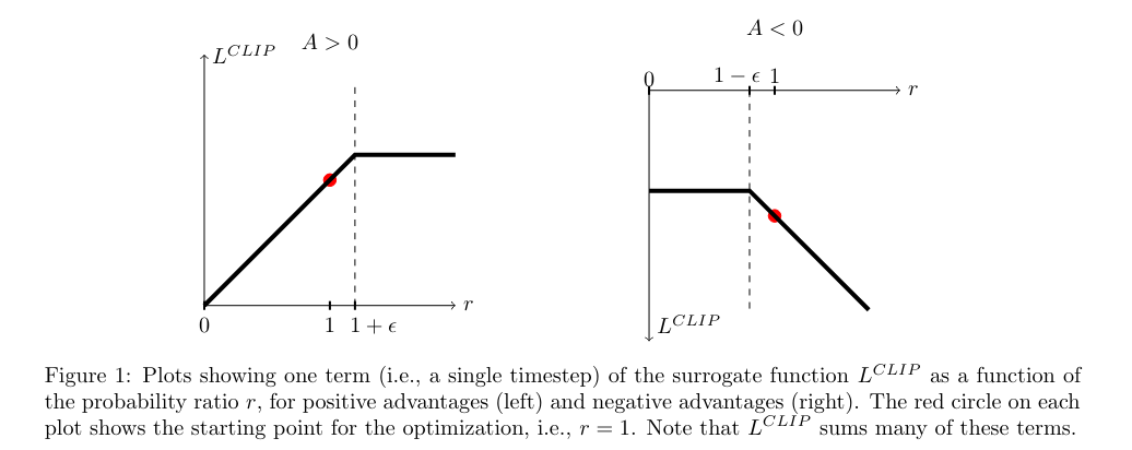
We will compare the updated policy to the previous one. Where this ratio would be too high – meaning we have deviated further away from the policy than we would like in the positive direction – we take a step of at most \(\epsilon\) in magnitude.

This safeguards us from making a large step in the parameter space away from our current policy. As discussed before, doing so would risk overshooting the area of quick improvement and might take us to regions where our policy becomes degenerate.

Since we use the policy to sample train data, we might not be able to recover from such a predicament!

Instead, we chose to take a smaller step in the hope that our policy continues to improve monotonically.

On the other hand, if we are fixing an issue with our policy where the ratio is smaller than 1 (policy before the update assigns a greater probability to a beneficial action than policy after the update), the step is unbounded.

In the negative direction, we are happy to move as far as indicated by the calculation:

Summary

Proximal Policy Optimization (PPO) has been a significant advancement in applying deep reinforcement learning to real-life scenarios.

OpenAI utilized PPO to train a system at an unprecedented scale called OpenAI Five, which successfully defeated the reigning Dota 2 champions. This showcased the potential of PPO in tackling complex strategic challenges.

Furthermore, PPO has seen widespread adoption in robotics, where it has been instrumental in devising effective control policies for robots. Its ability to handle continuous action spaces and stability during training has made it a popular choice for robotics applications.

Here is a quick recap of the method I generated with Claude Opus:

The key idea behind PPO is that it uses a single policy and performs multiple epochs of updates on the same batch of collected trajectories. The probability ratio is calculated between the current policy (being updated) and the policy used to collect the trajectories (before the update). This allows PPO to make conservative updates to the policy while still improving its performance.

By using a clipping function in the surrogate objective, PPO prevents the policy from changing too drastically in a single update, which helps to maintain stability during training. The clipping function limits the size of the policy update by constraining the probability ratio within a certain range.

Very excited to be including PPO in my toolbox!