Diving into Diffusion Policy with LeRobot

In a recent blog post, we looked at the Action Chunking Transformer (ACT).
At the heart of ACT lies an encoder-decoder transformer that when passed in
- an image
- the current state of the robot
- and an optional style variable
z
generates the next chunk_size number of actions.
But even the omnipowerful transformer is unable to produce actions out of thin air.
In ACT, we pass in learned embeddings into the decoder as input. As they travel up the decoder stack and are transformed in the context of the memory from the encoder, they turn into actions that make up the predicted trajectory.
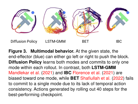
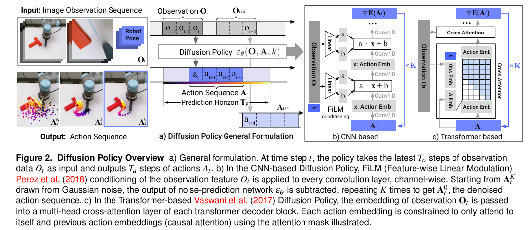
The Diffusion Policy, as outlined in the seminal "Diffusion Policy: Visuomotor Policy Learning via Action Diffusion" paper, takes a slightly different approach to manifesting the predicted actions.
Diffusion Policy starts with Gaussian noise instead of learned embeddings. It then iteratively removes the noise to arrive at the predicted actions.
In this blog post, we will explore the inner workings of this process by analyzing the code provided in LeRobot, a newly released library from Hugging Face.
Understanding the task at hand
We will train on the pusht dataset. The blue circle is the agent whose position is parametrized by the x and y coordinates of the center of the circle.
The goal is to push the light-gray T onto the light-green one.
The LeRobot library comes with everything we will need
- the
pushtdataset with 205 trajectories available from the Huggingface Hub - an easy-to-parse implementation of the Diffusion Policy
- an environment to evaluate our agent
- and example code making it very easy to get started with training
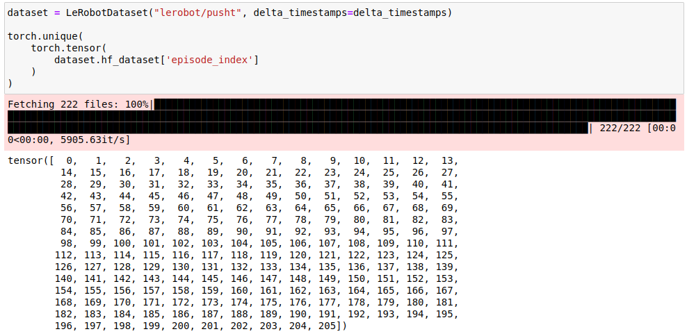
pusht dataset. The LeRobotDataset is a thin wrapper around the familiar Hugging Face datasets.Dataset that you can always drop down to via dataset.hf_datasetYou can also find the code for this blog post implementing the training in a jupyter notebook here.
Every journey begins with the first step
Let's first understand the data we will be training our policy on.
The LeRobotDataset features a very handy delta_timestamps functionality that defines the examples that will be returned.
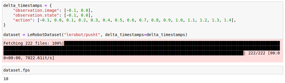
Above we specify that we would like our examples to contain:
observation.imageandobservation.statefrom the current timesteptand fromt-1(the offsets are given in seconds, but fromdataset.fpswe know-0.1sist-1)actionfrom timestepst-1tot+14
And this is what an example based on these specifications looks like:
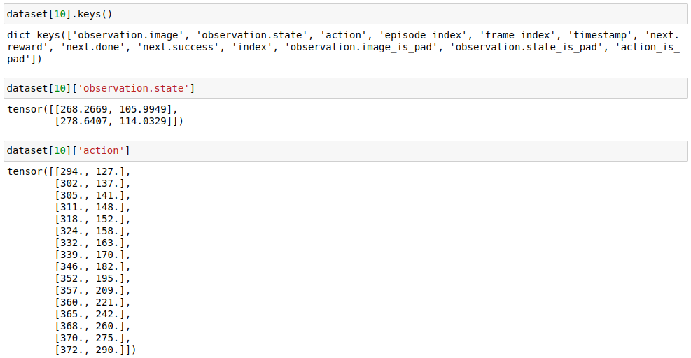
We can see that observation.state is different from action even for the first two overlapping time steps (t-1 and t).
This highlights an important aspect of the naming convention – state is the position the agent (or robot) finds itself in and action is the goal position of the agent (or robot).
action is the move command. By specifying the action, which is essentially the goal position, the agent begins moving toward the target location (or target joint position in the case of a robot) within the limits of its capabilities and the constraints of the environment (the movement is not instantaneous).
Although action and observation.state are represented in the same units, they have distinct meanings and serve different purposes.
The model's objective is to predict the action. By sending these predictions to the agent at the appropriate time steps, we aim to generate a trajectory that will complete the task.
Computing the loss
We now have a good overview of the information the policy operates on – so how do we generate predictions and calculate the loss during training?
At the heart of the Diffusion Policy is a 1D U-Net.
But before we can employ it we need to reshape our inputs into a format that it can operate on effectively.
We begin with the two images (observation.image from our batch). They are 96 pixels x 96 pixels with 3 channels.
We pass them through a resnet18 with the classification head removed and get back 512 channels (feature maps), each of dimensionality 3x3.
The interesting bit is what happens next. The authors chose to leverage SpatialSoftmax from "Deep Spatial Autoencoders for Visuomotor Learning".
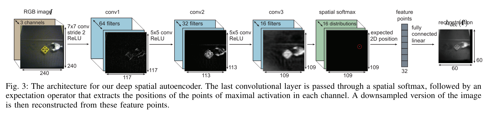
SpatialSoftmax takes the 512x3x3 input and reduces the number of channels to the desired number of keypoints (32 in our case) using convolutions.
It then applies a softmax over each channel. The softmax pushes most of the activations towards 0, while the highest value among the inputs is pushed towards 1.
Finally, the network performs a matrix multiplication between the unrolled attention vector obtained from the previous operation and a matrix of x and y coordinates.
This is how it looks in the code:
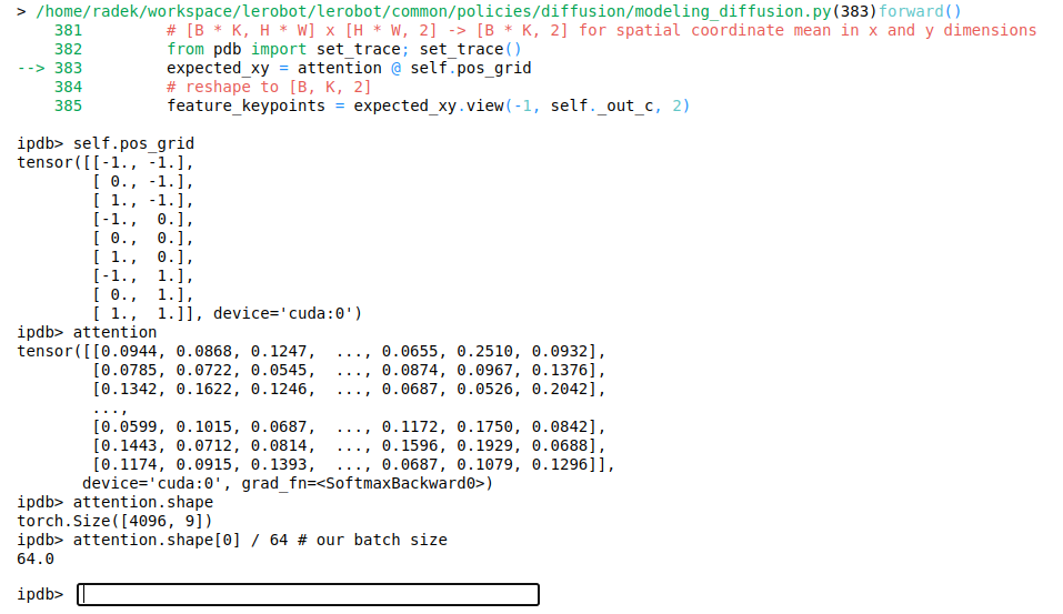
We have 4096 rows of attention (unrolled 3x3 feature maps that had softmax applied) as the batch size is 64 with each example consisting of 2 images, each with 32 key points (64x32x2 = 4096).
Using matrix multiplication, we take a weighted sum of the x and y coordinates in pos_grid by matrix multiplying it with the attention matrix.
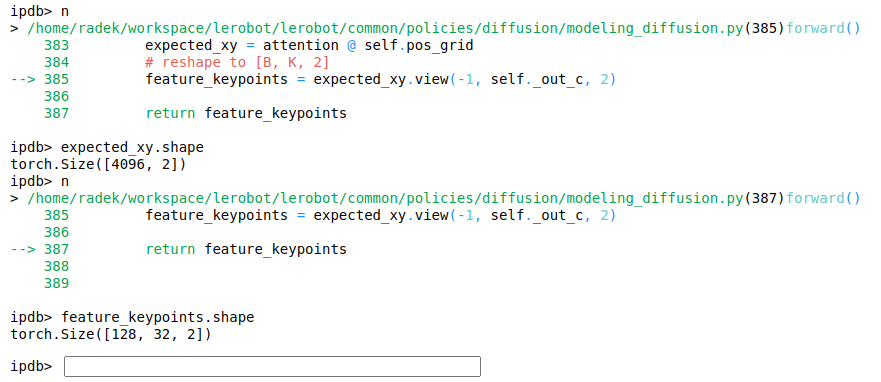
We obtain the corresponding keypoint coordinates for each row of attention and reshape them to the desired shape (32 keypoints per image, each consisting of 2 values – one for x, the other for y).
And the crazy thing is that... this works 🙂
The generated information for our model indicates the locations of points of interest across the 32 feature maps.
The softmax operation is differentiable, and multiplying it by the constants in the pos_grid doesn't change this property.
In the end, we take the coordinates, pass them via a linear layer, take a ReLU of the result, reshape the values, and obtain img_features of dimensionality [64, 2, 64] – 64 values for each of the 2 images across the batch of batch_size 64.
Phew... if you've made it to this point in the blog, congrats! 🥳 I have good news for you.
This has been the most complex operation we will look at in this blog post.
The rest of what the policy is doing should be much easier to follow as it doesn't venture that far off the beaten track as the SpatialSoftmax we looked at above.
Wrapping up input data processing
We now have the 32 key points, each consisting of 2 coordinates for the 2 images for each example.
That gives us 128 floats for each example (32x2x2) that represent the 2 images.
As the next step, we add the agent state at t-1 and at t. (it is impossible to infer the direction of the movement just from one data point, but with two you can!)
This brings us to 132 numbers per example (128 image descriptors + 2 keypoints x 2 coordinates).
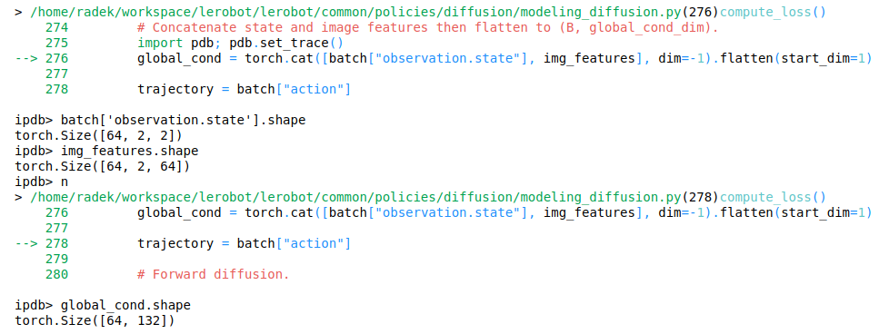
We will provide the 1D U-Net with the 132 numbers as the conditioning information (global_cond) to guide the trajectory generation.
It is worth emphasizing that the conditioning information originates from the past (t-1 and t). During the inference process, the action for the time step t-1 will have already been executed.
However, for training purposes, which involve calculating the loss and backpropagating gradients, we utilize the entire trajectory, consisting of the complete set of actions. For each example, this set of actions spans from step t-1 to t+14.
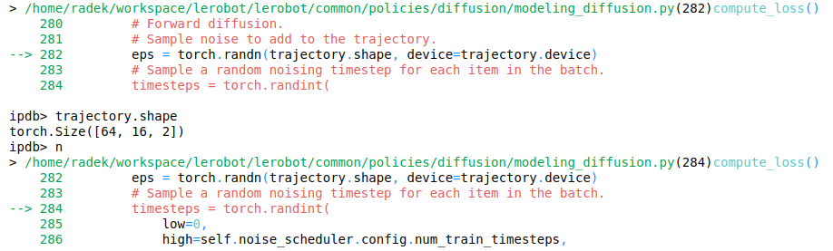
We grab our trajectory and generate Gaussian noise (sampled values from the Normal distribution) for each action.
During inference, using the default values, the DiffusionPolicy will remove noise over 100 iterations (denoising timesteps).
It will iteratively mutate variables sampled from the Normal distribution and at the end of the process we will receive the predicted actions.
In training, we want to approximate what the model will be asked to do during inference, and we approach this as follows.
For each example in the batch, we sample a random denoising step number (0 - 99).
We then add a variable amount of noise to each of the examples as per the noise_scheduler.
This way we obtain our starting condition (the noisy_trajectory), the input to our 1D U-net, with the noise that was added or the original trajectories (depending on the value of the prediction_type setting) constituting the targets.
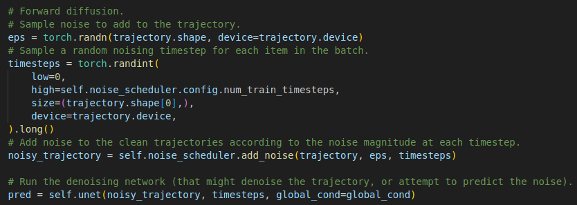
We pass the noisy_trajectories, the sampled timesteps and the global_cond conditioning information to our U-Net and obtain a prediction.
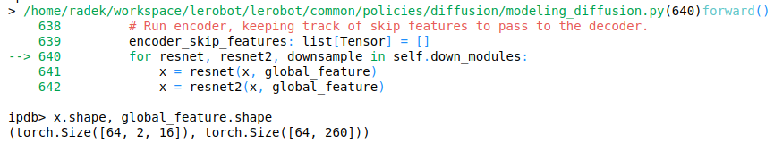
What does the U-Net do?
The U-Net architecture is a bit like an autoencoder as it also downsamples and upsamples the input.

But where an autoencoder aims to create a bottleneck in the middle, the U-Net does not.
The U-Net aims at efficiently and effectively processing and mutating the input based on the information it contains.
In our case, the U-Net will attempt to remove the noise from the passed in sequence of actions (or predict the noise, depending on the formulation we chose, as per the prediction_type parameter mentioned above).
As input, it receives the denoising timestep sampled for each example in the batch along with the noisy_trajectories (16 actions per each example, each with the x and y goal position coordinates).
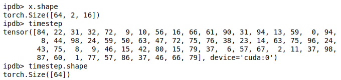
In addition to the diffusion time step information, the model will receive the global_cond, which includes the state and image features for time steps t-1 and t, processed into a vector with a dimensionality of 132.
The first order of business is to enhance the diffusion time step information (a single integer) with more meaningful representations.
One approach could be to utilize learnable embeddings for this purpose.
However, the authors of the Diffusion Policy paper employ a more elaborate technique, which presumably yields better results.
First, the integers representing the time step in the diffusion process get embedded using sinusoidal positional embedding. Each integer is expanded to 128 dimensions.
Intuitively, this makes sense. Essentially, instead of learning embeddings starting with random numbers (should torch.nn.Embedding be used), here we start with representations that are more alike the closer the steps are together (steps 46 and 47 will have positional encoding more similar than steps 46 and 58) and they retain this information during training.
Additionally, these sinusoidal embeddings don't only encode relative distance, but also the direction.
So why am I even bringing up torch.nn.Embedding and learnable embeddings in the first place?
Because while this formulation, I assume, is more tailored to the task, what we get in the end is still an embedding!
After being encoded using sinusoidal embeddings, the representation for our diffusion process timesteps is passed through two linear layers with a non-linearity in between!
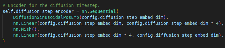
Whether we index into a set of learnable weights using one hot encoding (standard formulation of an embedding) or index into the learnable weights of a Linear layer by multiplying it with predefined vectors of floats, we still get an embedding in the end!
The only thing that remains now is to concatenate:
- image features for
t-1andt(128 dim) - states for
t-1andt(2 x 2 = 4 dim) - positional embeddings for the diffusion timestep (128 dim)
and we can feed this 260-dimensional vector as conditioning information to our U-Net!
And this is precisely what we do, passing along the noisy trajectories as inputs:
Interestingly enough, the conditioning information is passed directly to each layer of the U-Net (as opposed to being provided only to the initial layer).
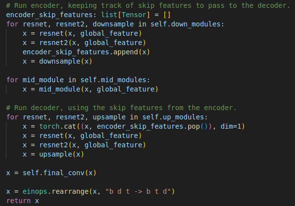
U-Net is rife in skip connections. Various improvements to the U-Net have been proposed via fusing layers, additional skip connections, etc, so it is no surprise that the conditional information might be iteratively fed to the model here.
It's akin to saying: "Hey model, I think this information is quite important, you better look at it some more". Additionally, this formulation also helps with gradient propagation and convergence.
Ultimately, we get the predictions from the U-Net.
At this point, there is nothing else to do but calculate the mean squared loss between the targets and outputs from our U-Net and backpropagate the loss (optionally masking out actions – padding – added at train time to bring examples to the desired shape).
n_obs_steps == 3 (O t-2 to 0t), n_action_steps == 4 (At to A t+3) and horizon == 10What happens at test time?
That is certainly a good question.
The composition of the training batch indicates that the inference process might not be as straightforward as expected. It involves a slightly more elaborate procedure than one might anticipate.
We pass the model two images and two states for t-1 and t (the number of used observations is a hyperparameter that we can tune, but as it impacts the model's architecture, it needs to be specified before training).
We process the state and the images as we had done during training.
For actions, we sample starting values from the Normal distribution and then use our trained U-Net to iteratively denoise the inputs, starting with reversing the last step of the diffusion process up to a total num_inference_steps (100 by default).
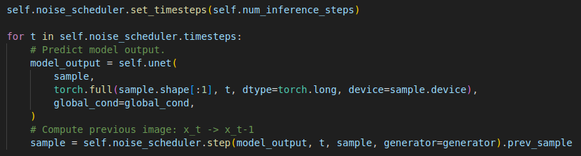
This generates actions for t-1 up to t+14. The t-1 action is from the past, so we discard it and only use n_action_steps, from t to t+n_action_steps-1, which defaults to 8.
Once we have exhausted our cached actions, we generate another set of actions from t-1 to t+14 and the process of selecting actions begins again.
Summary
Diffusion as a technique has taken various applications by storm.
The performance gains across many tasks are staggering, so it is a technique to look out for and add to your tool belt.
There have been many theoretical discussions about why diffusion works so well.
That is certainly an interesting debate, but at this point, I am more interested in pushing this method to the fullest and exploring its capabilities and limitations in various applications.
As such, to finish off this blog post, let me please share with you a couple of episodes recorded using an agent trained with lerobot and evaluated on the pusht environment converted by the HuggingFace team to the gym format.
We start with a success:
Here is where the agent fails. It runs out of time before accomplishing the success criteria – achieving 95% overlap between the two Ts.
What an unforgiving task and environment! 🙂
And in the below example, we see that hard work pays off! The agent completes the task just 30 actions shy of running out of time!
The planning needed to preposition the T for the follow-up sequence of movements is impressive
These are recordings from a training run I carried out using the default parameters. Please find the code I used for training here.
An enormous thank you to the LeRobot team for creating a wonderful resource to experiment with and learn from! 🙂