How to train your neural network

This blog post was originally published on Medium on 03/12/2018.

Imagine you live in the mountains. One of your kin has fallen sick and you volunteer to get medicine.

You stop by your house to grab the necessities — a map of the city along with a marble-shaped rock you claim brings you good fortune. You hop onto your dragon and fly north.

All that matters initially is a general sense of direction. The details on the ground are barely visible and you cover distance quickly.

As is widely known, dragons need a lot of space to land. You pick a nice landing spot just outside of a city and rent a horse from a nearby tavern.

You have to be more careful now — the horse is fast but if you want to get to the pharmacy before it closes you have to choose your direction more heedfully.

Once in the city, you take out the map, and taking big strides you run towards the main street. When finally there, you stop to catch your breath and look around.

Your objective is within sight and you casually stroll towards the entrance.

The journey you have just undertaken is very much like training a neural network. In order to converge to a good solution as quickly as possible we utilize different modes of movement by varying the learning rate.

The dragon is by far the fastest but it is also the least precise. While flying, the terrain looks roughly the same and you can only pick out major landmarks to use for navigation. This corresponds to training with a high learning rate.

The other extreme is walking slowly. You can observe all the details and pick your path nearly perfectly. This is our lowest learning rate.

If walking is so precise, why don’t we do it from start till finish? Because there is too much ground to cover and we would never get to the city in a reasonable time.

Why not fly all the way then? We would not be able to pinpoint our destination precisely from the air. Also, as our dragon is of considerable size, it might not be able to land close by to the target. The terrain in a city is quite rugged and the best we could probably do is pick a nice, flat rooftop to land on. Still, that would put us at some distance away from where we would like to be.

Our only hope is to combine training with a high and low learning rate to optimize both for speed and precision.

But how to go about it while training a neural network is not obvious. Below we will consider two ways of approaching this problem.

How to decay the learning rate

The most common way of decaying the learning rate is by hand. You train the network for some time and based on the results you make a decision whether to increase or decrease the learning rate. Rinse and repeat.

The whole process relies on intuition and it takes time to try things out.

Recently however a new method of decaying the learning rate was proposed[1]. In it, we provide an initial learning rate and over time it gets decayed following the shape of part of the cosine curve. Upon reaching the bottom we go back to where we started, hence the name — cosine annealing with restarts.

The diagram below contrasts using cosine learning rate decay with a manual, piece-wise constant schedule.

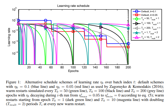
The new method has nice properties. First and foremost, we no longer have to worry about handcrafting a learning rate decay schedule. This saves us a considerable amount of time that we can spend elsewhere.

Furthermore, via jumping between lower and higher values of the learning rate in a non-linear fashion we hope to make it easier to navigate out of parts of the weight space that are particularly unfriendly to our optimizer.

Are those reasons good enough to warrant switching to the novel way of decaying the learning rate? Probably. But what about other important parameters like the training time or training accuracy?

Let’s look at both.

Comparison of training duration

We would like to measure how long it takes to fully train a model. But what does it mean for a network to be fully trained?

Is it something that you arrive at after training a model for some number of epochs? Or maybe when you achieve some validation set performance? Does it mean that with additional training we would not be able to achieve better results?

There are no easy answers to these questions. To have something more concrete I arbitrarily declare the finishing line to be an accuracy of 85% on the validation set.

To perform the experiment I train 40 resnet-20[2] models on CIFAR-10, 20 for each method of decaying the learning rate.

I use default parameters[2] that have been picked to work well with fixed learning rate decay. In many ways, I feel I am making life particularly hard for our automated annealing schedule.

And yet when I run the experiment, I get results as below.

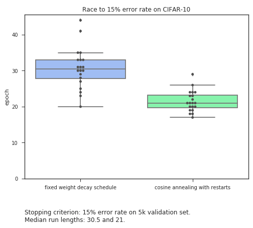
Cosine annealing wins the race by a significant margin. Also, quite importantly, there is a greater consistency to our results. This translates to greater confidence in the schedule to be able to produce consistently good results.

It might be quicker, but can it run the full distance? Is it able to get us to where we would like to be?

Accuracy of results

The promise of cosine annealing is that it should converge to solutions that generalize well to unseen data.

To perform an evaluation we can compare the results we get with the results achieved in the ResNet paper[2]. The authors trained for an equivalent of 182 passes through the training set achieving a test error of 8.75%.

We will perform 10 training runs with a cycle length of 7 and 14 (both divide 182 cleanly).

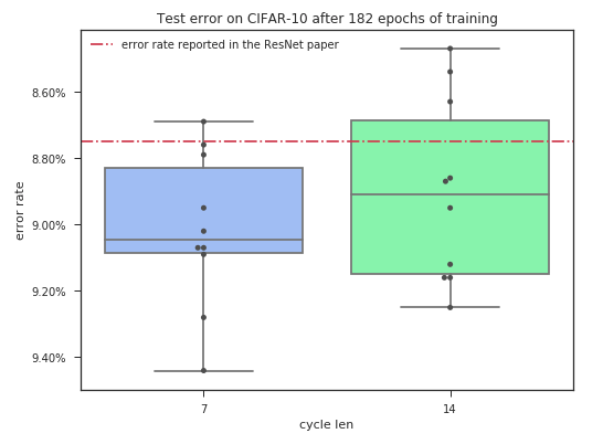
What is the significance of the results that we get? Does cosine annealing manage to deliver on its promise?

Summary

In my analysis, I have run cosine annealing with parameters that have been tuned over many years' worth of experiments to work well with decaying the learning rate manually.

Training all the way to completion with a starting learning rate of 0.1 is also undeniably not the right approach.

Probably the greatest concern is that I have not demonstrated how cosine annealing enriches the day to day workflow of a machine learning practitioner.

Running experiments is much quicker. I have more time I can spend on value add activities and do not have to occupy myself with chaperoning the training of a model.

It would be interesting to see how well cosine annealing can perform with settings devised specifically for it. But among all the unknowns I feel I have found the answer I have been looking for.

Given its inherent ability to save time and robustness to parameter values cosine annealing with restarts will most likely be my technique of choice across a wide range of applications.

[1] Stochastic Gradient Descent with Warm Restarts by Ilya Loshchilov and Frank Hutter

[2] Deep Residual Learning for Image Recognition by Kaiming He, Xiangyu Zhang, Shaoqing Ren, Jian Sun

[3] Cyclical Learning Rates for Training Neural Networks by Leslie N. Smith — a seminal paper that introduced the idea of cyclically varying the learning rate between boundary values

Tools used:

The Fastai library by Jeremy Howard and others

Implementation of Resnet-20 by Yerlan Idelbayev

You can find the code I wrote to run the experiments in my repository on GitHub.